I tried to implement a 2 layer (1 input and 1 hidden layer) neural network in R using gradient descent optimization. The steps followed for execution are similar to logistic regression only difference being the use of backpropagation which is used to adjust the weights in each layer of the network based on the rate of change of cost in the output layer. My primary objective for this post is to understand this backpropagation. Complete codes for this exercise can be found here.
Neural Nets - An Intro
The most basic type of neural net we use in machine learning mimics the neurons of a human brain. A neural network can be thought of layers of interconnected nodes. Every node in this net has a weight and bias. They act as a black box which takes some input and bias and based on its inherent weights and activation gives some output. These weights can be adjusted to tweak the output. One way of adjusting these weights is called backpropagation.
Analogy with logic gates
Logic gates in computer science also tend to be analogous to neural networks in some aspects.
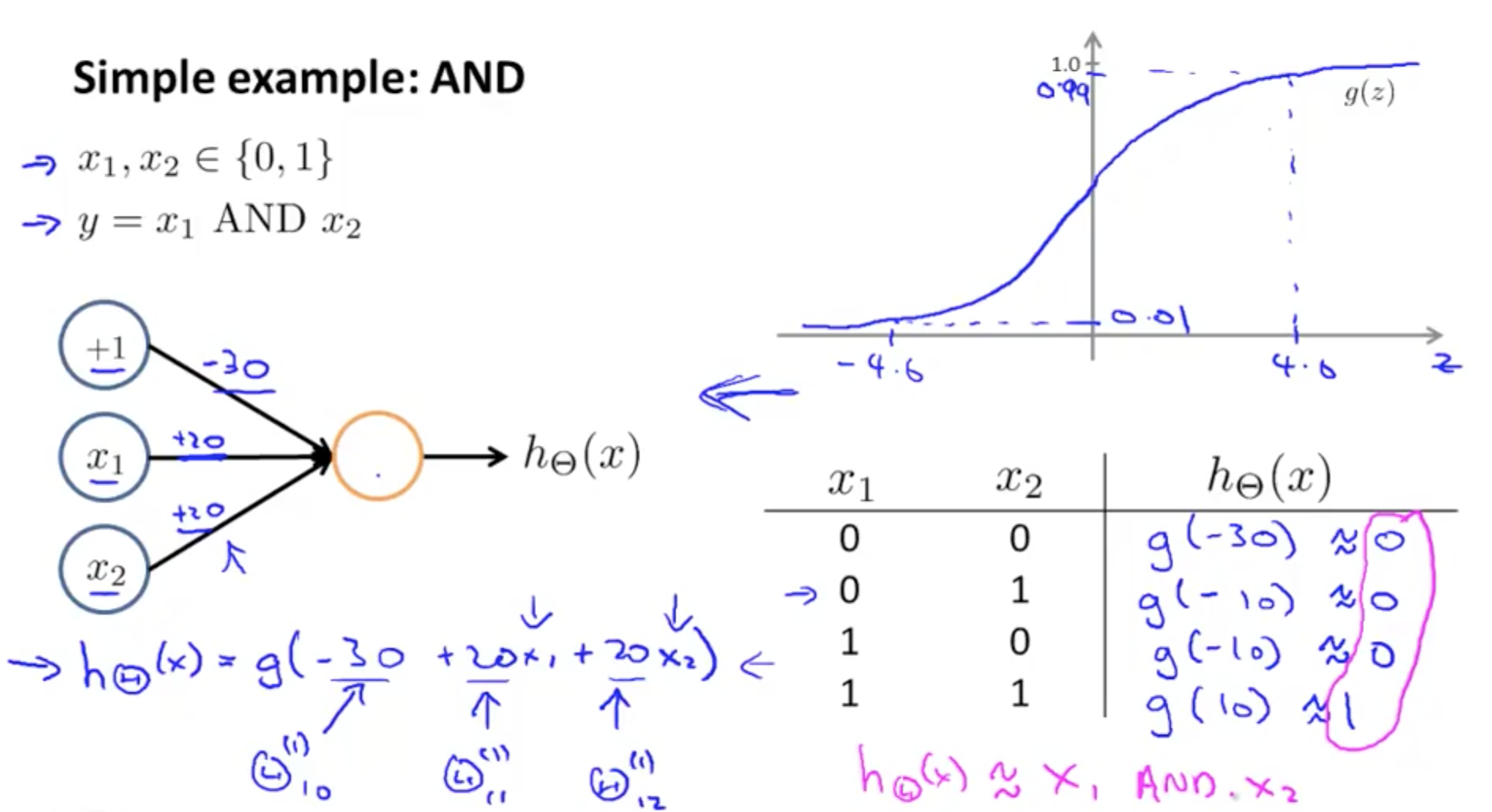
Here -30 is the bias and +20 and +20 are the weights. The activation used is a sigmoid function. This structure implements an AND gate. If I want to convert this into an OR gate I need to increase the value of +20, +20 to +40, +40 (greater than \( \lvert 30 \rvert \)). So one can change the weights and biases to obtain different outputs.
Steps for execution
1. Load dataset
Similar to logistic regression I have used the famous
iris dataset with 2 features Petal.Length and Petal.Width. My dependent variable will be
Species. I have also added an X intercept which will be 1. The data is split into train and test with a 70:30 ratio.
iris_data = iris[which(iris$Species %in% c("setosa", "versicolor")),]
iris_data$Species = ifelse(iris_data$Species == "setosa", 1, 0)

### adding X intercept to the data
iris_data$intercept = 1

iris_data = cbind(intercept = iris_data$intercept,
                  iris_data[,c("Petal.Length", "Petal.Width",  "Species")])

index = unlist(createDataPartition(iris_data$Species,p =  0.7))

train_x = as.matrix(iris_data[index,c("intercept", "Petal.Length", "Petal.Width")])
train_y = as.matrix(iris_data[index,c("Species")])

test_x = as.matrix(iris_data[-index, c("intercept", "Petal.Length", "Petal.Width")])
test_y = as.matrix(iris_data[-index, c("Species")])
2. Initialize \( \theta \) parameters for each layer
\( \theta_1 \) has the weights/gradient for the first layer which is the input layer. Number of nodes in the input layer must always be equal to the number of columns/features in the dataset. Therefore in my case the input layer has 2 nodes. The subsequent layers except the output layer can have any number of nodes. These are called the hidden layers of the network. The general rule of thumb is to have 1.5 times or number of nodes as the previous layer for each hidden layer. I assign random values between 0 to 1 from a normal distribution as weight/gradient for each node. Its values will change with each iteration of backpropagation.
num_labels = 2 # 1 and 2 in our case

m = dim(train_x)[1]
n = dim(train_x)[2]

## number of nodes in 1st layer/input layer must
## equal number of columns/ features of input data
layer1_nodes = ncol(train_x)

## this layer can have as many nodes as required
## rule of thumb is usually 1.5 times or equal number
## this is the hidden layer
layer2_nodes = trunc(ncol(train_x) * 1.5)

# final output layer nodes = number of labels
output_layer_nodes = num_labels

Theta1 = array(runif(n = gaussian(), min = 0, max = 1), c(layer2_nodes, layer1_nodes))

Theta2 = array(runif(n = gaussian(), min = 0, max = 1), c(output_layer_nodes, layer2_nodes+1))
3. Forward propagation
This is initial phase of a feed forward neural network. Data passes through the network using the initially assigned random weights till it reaches the output layer where we calculate the cost/error by comparing it with actual values.
3.a. Multiply independent variables x with the input layers \( \theta_1 \) (weights) and apply activation function
Similar to logistic regression I multiply the weights/gradient with the independent variables and apply an activation function. The activation in my case is sigmoid as I want to limit my output probability between 0 and 1.
## activation function - used to limit values between 0 and 1
sigmoid = function(x){
  return(1 / (1 + 2.71^-x))}

## input layer
a1 = train_x

z2 = a1 %*% t(Theta1)

a2 = sigmoid(z2)
Till this point every step is very similar to logistic regression. Which is the whole idea of neural networks, we can use any activation function and weights to achieve the desired output. Sigmoid gives us a linear decision boundary, but there are many other activation functions that give polynomial curves. Therefore, we can tune the complexity of our network based on the problem we want to solve.
Another thing to notice is that each individual node in a layer with its sigmoid activation acts as a logistic regression model. And one layer is just a combination of these individual models all working together to solve a complex problem.
3.b. Repeat the previous step for layer 2 and apply activation to the final output layer
We multiply the output of first layer with the weights of the second layer \( \theta_2 \). The final year applies the activation function to the output from the second hidden layer. No weight multiplication takes place in the final layer.
# second layer (hidden layer)
a2 = cbind(1, a2)

z3 = a2 %*% t(Theta2)

# third layer (output layer)
a3 = sigmoid(z3)
3.c. Calculate cost
Here I calculate difference between the result of the output layer and actual value \( y \). Since I am predicting a binary outcome I will use the same cost function I used for logistic regression which is logloss.
But the catch with neural networks is that because it is a combination of multiple logit regressors I will have to take the summation of the cost of each individual node in the output layer.
individual_train = array(0L, m)
individual_theta_k = array(0L, output_layer_nodes)
for(i in seq(1, m)){
  # for calculating innermost summation of cost (which is basically cost/error
  # for each node of the output layer wrt actual value)
  for(k in seq(1, num_labels)){
    individual_theta_k[k] = as.numeric(train_y[i,] == k)  * log(a3[i, k]) +
                          (1 - as.numeric(train_y[i,] == k)) * log(1 - a3[i, k])
  }
  # summation of errors at each label K for each input tuple/ row
  individual_train[i] = sum(individual_theta_k)
}
# summation of errors for all tuples
cost = -(1/m) * sum(individual_train)
cost
4. Backpropagation
This is where the learning in a neural network takes place. Backpropagation drives gradient descent. Based on the cost calculated in the output layer the weights in each layer are adjusted until the cost is minimized. The steps for doing backpropagation are as follows:
- Differentiate cost function. Taking a partial derivative of the cost function gives the rate of change of cost with an infinitesimally small change in \( \theta \). Similar to logistic regression this gives me the gradient vector to adjust the weights of the previous layer.
- Differentiate activation function of the hidden layers. Now consider that each of the hidden layers has a cost associated with it based on its weights which is contributing to the total cost in the output layer. I want to adjust weights in each layer in such a way that the next layer (including the output layer) will have minimum cost. How do I do this? By using the same logic I used in the output layer - I differentiate the function that has given me the output I need to pass to the next layer (in case of my output layer, the output is the final prediction) and this function for the each hidden layer is the activation function. Doing this I get the \( \theta \) adjustment for the previous layer. And this phenomenon propagates till the very first layer.
A more detailed explanation for this is available here.
4.a. Calculate gradient and adjust weights for each layer
My objective is to minimize this cost so I will use the partial derivative of my cost function to calculate by how much I need to change my \( \theta \) so that I am able to reduce the maximum cost.
## backpropagation (adjusting weights of previous layers wrt error in output layer)
## delta3 = error in output layer
## again done for each node in the layer
delta3 = array(0L, c(dim(a3)))
for(i in seq(1, m)){
  for(k in seq(1, num_labels)){
    delta3[i, k] = a3[i, k] - as.numeric(train_y[i,] == k)
  }
}

# this is the total error
delta3

# we will be taking a negative gradient of this error/ cost to calculate the
# direction of steepest descent and then adjust weights for each node of each layer
# accordingly

## used for backpropogation
sigmoidGradient = function(x){
  return(sigmoid(x) * (1 - sigmoid(x)))}
delta2 = (delta3 %*% Theta2[,2:ncol(Theta2)]) * sigmoidGradient(z2)

Theta1_grad = (1 / m) * t(delta2) %*% a1
Theta2_grad = (1 / m) * t(delta3) %*% a2
4.b Update \( \theta \)
Then I will update theta/gradients/weights for each layer according to my partial derivative. Here \( \alpha \) will be my step or learning rate by which I want to update my \( \theta \). Generally this \( \alpha \) must have a small value so that the gradient does not update frantically.
alpha = 0.001
Theta1 = Theta1 - alpha * Theta1_grad
Theta2 = Theta2 - alpha * Theta2_grad
Gradient descent
The repetition of forward and backpropagation in steps 1 to 4 to minimize cost is gradient descent. The following section shows the code for gradient descent:
cost = c()
num_labels = 2 # 0 and 1 in our case

m = dim(train_x)[1]
n = dim(train_x)[2]

## number of nodes in 1st layer/input layer must
## equal number of columns/ features of input data
layer1_nodes = ncol(train_x)

## this layer can have as many nodes as required
## rule of thumb is usually 1.5 times or equal number
layer2_nodes = trunc(ncol(train_x) * 1.5)

# final output layer nodes = number of labels
output_layer_nodes = 2

gradient_descent_for_nn = function(alpha, iterations, train_x, train_y)
{
  ## initialize theta (weights)

  Theta1 = array(runif(n = gaussian(), min = 0, max = 1), c(layer2_nodes, layer1_nodes))

  Theta2 = array(runif(n = gaussian(), min = 0, max = 1), c(output_layer_nodes, layer2_nodes+1))


  for(i in seq(1, iterations)){

    a1 = train_x

    z2 = a1 %*% t(Theta1)

    a2 = sigmoid(z2)

    a2 = cbind(1, a2)


    z3 = a2 %*% t(Theta2)

    a3 = sigmoid(z3)


    individual_train = array(0L, m)
    individual_theta_k = array(0L, output_layer_nodes)
    for(i in seq(1, m)){
      for(k in seq(1, num_labels)){
        individual_theta_k[k] = as.numeric(train_y[i,] == k)  * log(a3[i, k]) +
          (1 - as.numeric(train_y[i,] == k)) * log(1 - a3[i, k])
      }
      individual_train[i] = sum(individual_theta_k)
    }
    cost <<- c(cost, -(1/m) * sum(individual_train))
    # cost = c(cost, cost)
    # print(cost)


    delta3 = array(0L, c(dim(a3)))
    for(i in seq(1, m)){
      for(k in seq(1, num_labels)){
        delta3[i, k] = a3[i, k] - as.numeric(train_y[i,] == k)
      }
    }

    # delta3


    # delta2 = Theta2*delta3 * (derivative of activation function, which is sigmoid)
    # delta2 = Theta2*delta3 * a3 * (1 - a3)

    delta2 = (delta3 %*% Theta2[,2:ncol(Theta2)]) * sigmoidGradient(z2)

    Theta1_grad = (1 / m) * t(delta2) %*% a1
    Theta2_grad = (1 / m) * t(delta3) %*% a2

    # alpha = 0.001
    Theta1 = Theta1 - alpha * Theta1_grad
    Theta2 = Theta2 - alpha * Theta2_grad

  }
  return(list(Theta1, Theta2))

}


alpha = 0.01
## keep changing epochs, more epochs = more steps towards minimum cost
epochs = 3000

thetas = gradient_descent_for_nn(alpha, epochs, train_x, train_y)

plot(cost)


h1 = sigmoid(test_x %*% t(thetas[[1]]))
h2 = sigmoid(cbind(1, h1) %*% t(thetas[[2]]))


preds = apply(h2, 1, function(x) which(x == max(x)))

confusionMatrix(as.factor(preds), as.factor(test_y))
## 100% accuracy
One way to track the success of gradient descent is to check if our cost reduces with each iteration. The graph should follow an elbow curve shown here.
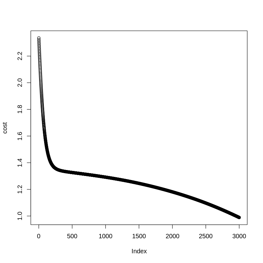
If no significant reduction is observed even after multiple iterations it is understood that there is something wrong with the network setup or data and the model is not learning resulting in a mediocre model.