This is an implementation of the logistic regression assignment from Andrew Ng’s machine learning class. Since the original implementation of these assignments is in Octave, and because I am more comfortable with R I tried implementing the same using R. No external libraries are used in this exercise as I wanted to build everything from scratch. Complete codes for this exercise can be found here.
Logisitic Regression - An Intro
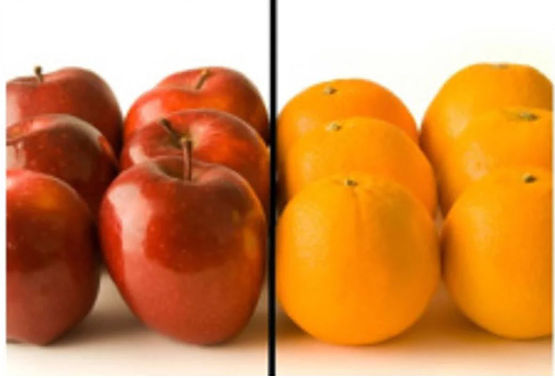
Logistic regression is one of the basic classification algorithms used in classical machine learning. Where I try to separate 2 different types of elements using a decision boundary in an n-dimensional space. The decision boundary is created in such away that it should completely separate the elements and no element of one type should be present with the element of another type (eg. the organization of apples and oranges in fruit basket is separated from one another using a cardboard strip. This cardboard strip acts as a decision boundary).
Decision Boundary
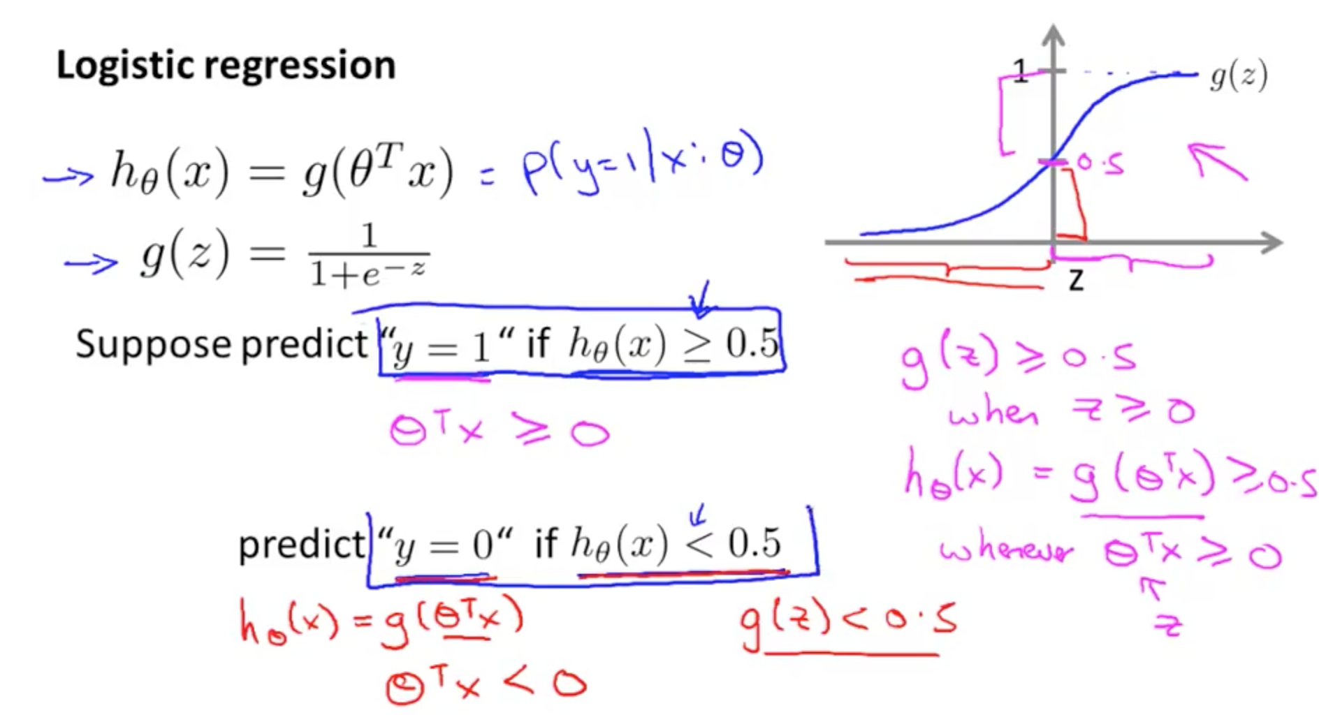
There are many ways to create this decision boundary. The most basic method is to fit a line through my data so that there is minimum distance between the data points and my fitted line. And based on this fitted line I will be able to obtain my decision boundary. Eg. Consider that my fitted curve is a sigmoid function, then for any value where \( h _\theta(x) \) >= 0.5, \( y \) = 1 and for \( h _\theta(x) \) < 0.5, \( y \) = 0. Given a value of \( x \), \( h _\theta(x) \) is the hypothesis or “probability” of \( y \) being 1 or 0. And \( h _\theta() \) is the activation or model used to map \( y \) to \( x \), which in this case is a sigmoid function.
Steps for execution
1. Load dataset
I have used the famous iris dataset with 2 features Petal.Length and Petal.Width. My dependent variable will be
Species. I have also added an X intercept which will be 1. The data is split into train and test with a 70:30 ratio.
iris_data = iris[which(iris$Species %in% c("setosa", "versicolor")),]
iris_data$Species = ifelse(iris_data$Species == "setosa", 1, 0)

### adding X intercept to the data
iris_data$intercept = 1

iris_data = cbind(intercept = iris_data$intercept,
                  iris_data[,c("Petal.Length", "Petal.Width",  "Species")])

index = unlist(createDataPartition(iris_data$Species,p =  0.7))

train_x = as.matrix(iris_data[index,c("intercept", "Petal.Length", "Petal.Width")])
train_y = as.matrix(iris_data[index,c("Species")])

test_x = as.matrix(iris_data[-index, c("intercept", "Petal.Length", "Petal.Width")])
test_y = as.matrix(iris_data[-index, c("Species")])
2. Initialize \( \theta \) parameters
\( \theta \) is the gradient. Start by assigning random values to this vector. Its values will change with each iteration of gradient descent.
init_theta = as.matrix(c(0, 0.5, 0.5), 1)
3. Multiply independent variables x with \( \theta \) (weights) and apply activation function
Here I multiple the weights/gradient with the independent variables and apply an activation function. The activation in my case is sigmoid as I want to limit my output probability between 0 and 1. This will give me my \( h_\theta(x) \) which is the function/model that maps \( x \) (independent variable) to \( y \) (dependent variable).
z1 = train_x %*% c(t(init_theta))

## activation function - used to limit values between 0 and 1
sigmoid = function(x){
  return(1 / (1 + 2.71^-x))}

hthetax = mapply(sigmoid, z1)
4. Calculate cost
Here I calculate difference between my predicted \( h_\theta(x) \) and actual value \( y \). This is calculated using a cost function. In my case the cost function is logarithmic loss or logloss.
logloss_cost = function(y, yhat){
  return(-(1 / nrow(y)) * sum((y*log(yhat) + (1 - y)*log(1 - yhat))))}

logloss_cost(train_y, hthetax)
5. Calculate gradient
My objective is to minimize this cost so I will use the partial derivative of my cost function to calculate by how much I need to change my \( \theta \) so that I am able to reduce the maximum cost. Here \( \alpha \) will be my step or learning rate by which I want to update my \( \theta \).
## gradient calculation
alpha = 0.01
theta_iter = alpha/nrow(train_x) * (t(train_x) %*% c(hthetax - train_y))
6. Update \( \theta \)
Then I will update theta according to my partial derivative.
## updating gradient
init_theta = init_theta - theta_iter
init_theta
Gradient descent
The repetition of steps 1 to 6 to minimize cost is termed as gradient descent. The following section shows the code for gradient descent:
cost = c()
gradient_descent_for_logloss = function(alpha, iterations, initial_theta, train_x, train_y)
{
  ## initialize theta (weights)
  theta = initial_theta
  for(i in seq(1, iterations)){

  z1 = train_x %*% c(t(theta))

  ## apply activation
  hthetax = mapply(sigmoid, rowSums(z1))

  ## calculating cost J(theta)
  cost <<- c(cost, logloss_cost(train_y, hthetax))

  ## gradient calculation
  ## using derivative of cost function J(theta)
  theta_iter = alpha/nrow(train_x) * (t(train_x) %*% c(hthetax - train_y))

  ## gradient update
  theta = theta - theta_iter

  slope = theta[2]/(-theta[3])
  intercept = theta[1]/(-theta[3])
  plot(iris_data$Petal.Width, iris_data$Petal.Length)
  abline(intercept, slope)
  Sys.sleep(0)

  }
  return(theta)

}
alpha = 0.01
## keep changing epochs, more epochs = more steps towards minimum cost
epochs = 600

thetas = gradient_descent_for_logloss(alpha, epochs, as.matrix(c(0, 0.5, 0.5), 1), train_x, train_y)

thetas

################################################

## predicting using theta values
z_op = test_x %*% c(t(thetas))

pred_prob = mapply(sigmoid, z_op)

preds = ifelse(pred_prob > 0.5, 1, 0)

confusionMatrix(as.factor(preds), as.factor(test_y))
## 96% accuracy